Thursday, June 7, 2018

Why p-values are Bad for Science

This post is the fifth in a series of seven posts in which I am arguing against the use of p-values for reporting the results of statistical analysis. You can find a summary of my argument and links to the other posts in the first post of the series. In this post, I present why I think p-values are bad for science.

The problems that I have with p-values and NHST are not minor quibbles. They unfortunately cut to the core of scientific practice. They affect the quality of reported and published scientific evidence, they perturb in major ways the process of accumulation of knowledge and eventually they might undermine the very credibility of our scientific results.

I can see two major detrimental consequences to the use of p-values and NHST:
  1. Publication bias: published results overestimate the true effects, by a large margin, with published results being 1.5 to 2 times larger than the true effects on average.
  2. Imprecision: published results have low precision, with a median signal to noise ratio of 0.26.

Publication bias


Publication bias operates in the following way: if editors decide to publish only statistically significant results, then the record of published results will be an overestimate of the true effect, as we have seen in the previous post of the series. If a true effect is small and positive, published results will overestimate it.

This means that if the true effect is nonexistent, only positive and negative studies showing that it exists and is large will be published. We will get either conflicting results or, if researchers favor one direction of the effect, we might end up with evidence for an effect that is not there.

There are actually different ways publication bias can be generated:
  • Teams of researchers compete for publication based on independent samples from the same population. If 100 teams compete, on average, 5 of them will find significant results even if the true effect is non-existent. Depending on the proportion of true effects that there is to discover, it might imply that most published research findings are false
  • Specification search is another way a team can generate statistically significant results. For example, by choosing to stop collecting new results once the desired significance is reached, choosing to add control variables or changing the functional form. This does not have to be conscious fraud, but simply a result of the multiple degrees of freedom that researchers have, which generate what Andrew Gelman and Eric Loken call "the garden of forking paths." In a pathbreaking paper in psychology, Joseph Simmons, Leif Nelson and Uri Simonsohn showed that leveraging on degrees of freedom in research, it is very easy to obtain any type of result, even that listening to a given song decreases people's age.
  • Conflicts of interest, such as in medical sciences where labs have to show efficiency of drugs, might generate a file drawer problem, where insignificant or negative results do not get published.
Do we have evidence that publication bias exists? Unfortunately yes, massive, uncontroversial evidence. The evidence on publication bias comes from replications attempts and meta-analysis.

Evidence of publication bias from replications


Replications consists in trying to conduct a study similar to a published one, but on a larger sample, in order to increase precision and decrease sampling noise. After the replication crisis erupted in their field, psychologists decided to conduct replication studies. The Open Science Collaboration published in Science in 2015 the results of 100 replication attempts. What they found was nothing short of devastating (my emphasis):
The mean effect size (r) of the replication effects (Mr = 0.197, SD = 0.257) was half the magnitude of the mean effect size of the original effects (Mr = 0.403, SD = 0.188), representing a substantial decline. Ninety-seven percent of original studies had significant results (P < .05). Thirty-six percent of replications had significant results; 47% of original effect sizes were in the 95% confidence interval of the replication effect size.
Here is a beautiful graph summarizing the terrible results of the study:
The results in red are results that were statistically significant in the original study but that were not statistically significant in the replication.

It seems that classical results in psychology such as priming and ego depletion do not replicate well, at least under some forms. The replication of the ego depletion original study was a so-called multi-lab study where several labs ran a similar protocol and gathered their results. Here is the beautiful graph summarizing the results of the multi-lab replication with the original result on top:

The original study was basically an extreme observation drawn from a distribution centered at zero, or very close to zero, a clear sign of publication bias at play.

What about replication in economics? Well, there are several types of replications that you can run in economics. First, for Randomized Controlled Trials (RCTs), either run in the lab or in the field, you can, as in psychology, run another set of experiments similar to the original. Colin Camerer and some colleagues did just that for 11 experimental results. Their results were published in science in 2016 (emphasis is mine):
We find a significant effect in the same direction as the original study for 11 replications (61%); on average the replicated effect size is 66% of the original.
So, experimental economics suffers from some degree of publication bias as well, although apparently slightly smaller than in psychology. Note however that the number of replications attempted is much smaller in economics, so that things may get worse with more precision.

I am not aware of any replication in economics of the results of field experiments, but I'd be glad to update the post after being pointed to studies that I'm unaware of.

Other types of replication concerns non experimental studies. In that case, replication could mean trying to replicate the same analysis with the same data, in search of a coding error or of debatable modeling choices. What I have in mind would rather be trying to replicate a result by looking for it either with another method or in different data. In my own work, we are conducting a study using DID and another study using a discontinuity design in order to cross check our results. I am not aware of intents to summarize the results of such replications, if they have been conducted. Apart from when it is reported in the same paper, I am not aware of researchers trying to actively replicate the results of quasi-experimental studies with another method. Again, it might be that my knowledge of the literature is wanting.

Evidence of publication bias from meta-analysis


Meta-analysis are analysis that regroup the results of all the studies reporting measurements of a similar effect. The graph just above stemming from the multi-lab ego-depletion study is a classical meta-analysis graph. In the bottom, it presents the average effect taken over studies, weighted by the precision of each study. What is nice about this average effect is that it is not affected by publication bias, since the results of all studies are presented. In order to guarantee that there is no selective publication, authors of the multi-lab study preregistered all their experiments and committed to communicate the results of all of them.

But absent a replication study with pre-registration, estimates stemming from the  literature might be affected by publication bias, and the weighted average of the published impacts might overestimate the true impact. How can we detect whether it is the case or not?

There are several ways to detect publication bias using meta-analysis. One approach is to look for bumps in the distribution of p-values or of test statistics around the conventional significance thresholds of 0.05 or 1.96. If we see an excess mass above the significance threshold, that would be a clear sign of missing studies with insignificant results, or of specification search transforming p-values from 0.06 into 0.05. Abel Brodeur, Mathias Lé, Marc Sangnier and Yanos Zylberberg plot the t-statistics for all empirical papers published in top journals in economics between 2005 and 2011:
There is a clear bump in the distribution of test statistics above 1.96 and a clear trough below, indicative that some publication bias is going on.


The most classical approach to detect publication bias using meta-analysis is to draw a funnel plot. A funnel plot is a graph that relates the size of the estimated effect to its precision (e.g. its standard deviation). As publication bias is more likely to happen with imprecise results, a deficit of small imprecise results is indicative of publication bias. The first of the three plots below on the left shows a regular funnel plot, where the distribution of results is symmetric around the most precise effect (ISIS-2). The two other plots are irregular, showing clear holes at the bottom and to the right of the most precise effect, precisely where imprecise small results should be in the absence of publication bias.


More rigorous tests can supplement the eyeball examination of the funnel plot. For examples, one can regress the effect size on precision or on sampling noise. A precisely estimated nonzero correlation would signal publication bias. Isaiah Andrews and Maximilian Kasy extend these types of tests to more general settings and apply them to the literature on the impact of the minimum wage on employment, and find, as previous meta-analysis already did, evidence of some publication bias in favor of a negative employment effect of the minimum wage.

Another approach to the detection of publication bias in meta-analysis is to compare the most precise effects to the less precise ones. If there is publication bias, the most precise effects should be closer to the truth and smaller than the less precise effects, which would give an indication of the magnitude of publication bias. In a recent paper, John Ioannidis, T. D. Stanley and Hristos Doucouliagos estimate the size of publication bias for:
159 empirical economics literatures that draw upon 64,076 estimates of economic parameters reported in more than 6,700 empirical studies.
They find that (emphasis is mine):
a simple weighted average of those reported results that are adequately powered (power ≥ 80%) reveals that nearly 80% of the reported effects in these empirical economics literatures are exaggerated; typically, by a factor of two and with one‐third inflated by a factor of four or more.

Still another approach is to draw a p-curve, a plot of the distribution of statistically significant p-values, as proposed by Joseph Simmons, Leif Nelson and Uri Simosohn. The idea of p-curving is that if there is a real effect, the distribution of significant p-values should lean towards small values, because they are much more likely than large values close to the 5% significance threshold. Remember the following plot from my previous post on significance testing:
Most of the p-values should be larger than 0.05 if the true distribution is the black one, since most samples will produce estimates located to the right of the significance threshold. If there is no real effect, on the contrary, the distribution of p-values is going to be flat, by construction. Indeed, the probability of observing a p-value or 5% or less is 5% while the probability of observing a p-value of 4% or less is 4%, hence, the probability of observing a p-value between 5% and 4% is exactly 1% in the absence of any real effect, and it is equal to the probability of observing a p-value between 4% and 3% and so on. When applied to the (in)famous "Power Pose" literature, p-curve is flat:


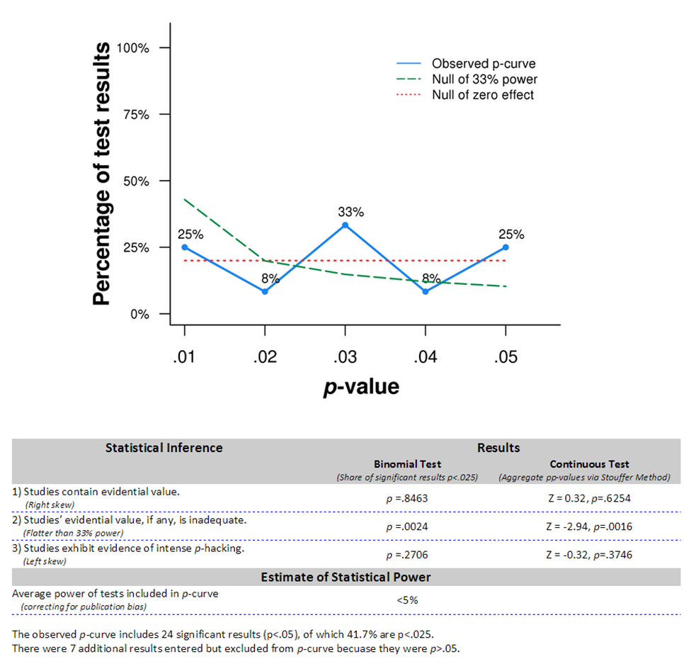
The flat p-curve suggests that there probably is no real effect of power pose, at least on hormone levels, which has also been confirmed by a failed replication. Results from a more recent p-curve study of Power Pose claims evidence of real effects, but Simmons and Simosohn have raised serious doubts about the study.

There is to my knowledge no application of p-curving to empirical results in economics.

Underpowered studies


Another problem with p-values and Null Hypothesis Significance Testing (NHST) is that they are used to perform a power analysis in order to select the adequate sample size before running a study. The usual practice is to choose sample size so as to have 80% chance of detecting an effect at least equal to a minimum a priori postulated magnitude (a.k.a. the minimum detectable effect) using NHST with a p-value of 5%.

The problem with this approach is that it focuses on p-values and test statistics and not on precision or sampling noise. As a result, the results obtained using classical power analysis are not very precise. One can actually show that the corresponding signal to noise ratio is equal to 0.71, meaning that noise is still 25% bigger than signal.

With power analysis, there is no incentive to collect precise estimates by using large samples. As a consequence, the precision of results published in the behavioral sciences has not increased over time. Here is a plot of the power to detect small effect sizes (Cohen's d=0.2) for 44 reviews of papers published in journals in the social and behavioral sciences between 1960 and 2011 collected by Paul Smaldino and Richard McElreath:


There is not only very low power (mean=0.24) but also no increase over time in power, and thus no increase in precision. Note also that the figure shows that the actual realized power is much smaller than the postulated 80%. This might be because no adequate power analysis was conducted in order to help select the sample size for these studies, or because the authors selected medium or large effects as their minimum detectable effects. Whether we should expect small, medium or large effects in the social sciences depends on the type of treatment. But small effects are already pretty big: they are as large as 20% of the standard deviation of the outcome under study.

John Ioannidis and his coauthors estimate that the median power in empirical economics is 18%, which implies a signal to noise ratio of 0.26, meaning that the median result in economics contains four times more noise than it has signal.

Wednesday, June 6, 2018

My Problems with p-values

This post is the fourth in a series of six posts in which I am arguing against the use of p-values for reporting the results of statistical analysis. You can find a summary of my argument and links to the other posts in the first post of the series. In this post, I present my problems with p-values. 

What are my problems with p-values? Oyy, where to start? Here are four reasons why I hate p-values and NHST:
  1. Science is not about making decisions each time you see a new sample. NHST and p-values are not designed for scientific inquiry but for industrial decisions.
  2. In general, scientists interpret statistically significant effects as equal to the true effect while non-statistically significant results are interpreted as zeroes. Both of these interpretations are deeply WRONG.
  3. Statistically significant results are biased.
  4. Marginally significant results are very imprecise.

NHST and p-values are not designed for scientific inquiry but for industrial decisions


NHST and p-values are not adapted to scientific inquiry but to industrial practice. In order to explain to you why this is the case, let me tell you a story.  (I do not know if this story is 100% true or only apocryphal, but I'm pretty sure I read it in one of Stephen Stigler's books or in Hald's History of Mathematical Statistics. Whether the story is accurately true or not does not really matter though, since it is mostly there to illustrate the context of use of NHST and p-values).

The inventor of the significance test is William S. Gosset, better know under his pen-name of Student (he was so humble that he considered himself a student of the great statisticians of his day, especially Karl Pearson). William Gosset wrote under a pen-name because he was not an academic but was working for a private firm, actually the famous Guiness beer factory. Gosset designed the testing procedure in order to solve a very practical problem that he faced at his job. Everyday, a new batch of grain would come in. Before sending the grain into production, Guiness employees would take a sample of the grain (let's say ten small samples taken in random parts of the batch) in order to assess its quality. They would estimate the quality of the grain in each of the samples for a characteristic important for brewing. Based on the sample, they would have to decide whether to discard the batch or put it under production. The problem is that the sample is a noisy estimate of the quality of the batch. If the batch was bad, but they wrongly decided to put it into production, they would lose money. If the batch was good and they decided to discard it, they would also lose money. You recognize the errors of the second and first type of test statistics. So Gosset had to make a choice, everyday, based on a sample, to discard or accept a batch of grain. He devised a procedure that would minimize the risk of discarding a good batch under a fixed probability of discarding a bad one. The procedure simply used a test statistic: compute the value of the test statistic under the assumption that the batch is good. Compute its p-value. Discard the batch if the p-value is smaller than 0.05.

Gosset's procedure (and test statistics in general) makes a lot of sense in an industrial context. There is repeated sampling and actual decisions made at each sample repetition. Test statistics are perfectly adapted to this problem. Science is a very different problem altogether. There is no repeated sampling. We do not take a decision after each sample repetition. We do not need a procedure to help us make this decision. Fisher was the one who adapted Gosset's idea and translated it to scientific practice. He devised p-values as a means to estimate the strength of the evidence in favor of an assumption. He suggested that we could say that under 5%, the bulk of the evidence could be considered overwhelmingly against the assumption. But he never made this threshold a magical threshold. What made this threshold magical was the procedure of decision attached to statistical testing, that Neyman and Pearson coined after Gosset. But, again, this procedure was adapted to an industrial context of repeated decisions, not to scientific inquiry.

NHST and p-values give a false cutoff sense of confidence


The problem with using test statistics in science is that they focus our attention on the position of our results with respect to a cutoff. Have you ever noticed how much more excited you feel when your results cross the 5% significance threshold? How disappointed you are when they are just below? We also tend to radically alter our reporting of a result when it is statistically significant. For example, if  a coefficient is statistically different from zero, we are happy and we report it as being a positive effect. If the result is not statistically different from zero, we report as being insignificant, and in general we consider it as good as zero. This is something every single one of us has felt.

And this is wrong. It proves a deep misunderstanding of what sampling noise really is and what statistical testing is all about.


Look for example at samples 27 and 28 when N=1000 on the figure above. With sample 27, you have a treatment effect estimated at around 0.18, significantly different from zero at the 5% level. So two stars significance. Great. You tend to interpret this result as a 0.18 positive significant treatment effect, and you are going to remember 0.18. With sample 28, you have a a treatment effect estimated at around 0.17, not significantly different from zero at the 5% level. You tend to interpret this result a non-significant treatment effect, and in general you are going to remember it as a zero. But the two samples contain exactly the same objective information: the confidence interval for the effect is large, ranging from very small (zero or slightly negative) to large.

You cannot change your opinion on a program because some random noise has marginally changed your estimator so that its test statistic falls just above or just below 1.96. Nothing has objectively changed between these two samples. The only reason why we would need to choose a cutoff and change our minds when crossing this threshold is because we want to make a decision. But there is no decision to make. So we should consider the two samples as bringing exactly the same information: either a very small effect (positive or negative) or a very large positive one.

But the 95% confidence interval for sample 28 tells us that the effect might be negative whereas that is not the case for sample 27. Doesn't it count for something? No, and for two reasons. First, a very small effect, positive or negative, is just small and does not have important consequences in the real world. Second, even if it does, your precision does not allow you to conclude anything certain. Probability distributions are continuous here, and the change of probability for the treatment effect being below zero from sample 27 to sample 28 is marginal, extremely small. You can see that if you use the 99% confidence interval. Then sample 27 also contains zero and small negative effects.

Look now at samples 18 and 19 of the same graph. The effects there are small and zero is well within the confidence bands, so a statistical test would just give you an insignificant estimate. In general, you will interpret this as a zero. But this would be wrong. Completely wrong actually, since the true treatment effect is actually 0.18. And the objective information from the confidence interval tells you just that: 0.18 is well within the confidence bands too.

Stick with the objective information. Tests focus your attention on details and marginal changes and cutoff decisions instead of looking at sampling noise objectively. Tests are used as a way to gain false certainty in front of sampling noise. No statistical test can get rid of sampling noise.
 

Statistically significant treatment effects are biased


One very annoying property of statistically significant results is that they are always biased upwards, especially if sampling noise is large (and thus especially if sample size is small). Look again at the figure above. With N=100, the estimates that are statistically different from zero at the 5% level are 2 to 2.5 bigger than the true effect. With N=1000, not all statistically significant results overestimate the true effect but most do.

That statistically significant results are biased upwards is a mechanical consequence of NHST. In order to shed more light on this, let's compute the p-values for the two-sided t-test that the treatment effect is zero for all our Monte Carlo samples using the CLT-based estimates of sampling noise. The figure below presents the results.

You can see that with N=100, treatment effects are significant at the 5% level only when they are at least bigger than 0.3 (the 5% threshold is the blue line on the graph, the red line is the threshold for 1% significance). Remember that the true effect is 0.18! With N=1000, samples with an estimated effect smaller than 0.1 are never significant at the 5% level. As a consequence, if you take the average of the statistically significant effects overestimate the true effect by a large amount: with N=100, statistically significant effects are on average double than the truth, whereas with N=1000, they are roughly 50% bigger.

Note that there is no such problem for larger sample sizes, where all results are statistically significantly different from zero. Actually, we should expect some estimates to be close to zero, but the probability that it happens is so small that it has no practical effect. People accustomed to p-values are thrown off when using large sample sizes where everything is significant at conventional levels. This is actually a funny consequence of people not understanding sampling noise and test statistics: the fact that everything is significant means that uncertainty about parameter values has decreased and that you can actually look at the magnitudes of the coefficients, not whether they are different from zero.


Marginally significant results are very imprecise


Another related very unfortunate consequence of p-values is that results that are marginally significant at the 5% level have are very imprecise: their signal to noise ratio is equal to 0.5, meaning that there twice as much noise as there is signal. This is a very simple consequence of using NHST. Remember that scientists consider a result to be significant at 5% when the ratio t=|x|/se(x) is superior to 1.96. Now, signal to noise ratio can be defined as s/n=|x|/y, with y the width of the 95% confidence interval. Remember that with a normal distribution, we have se(x)=y/(2*1.96). As a consequence, t~1.96 -> s/n~0.5.

A related consequence of using NHST is that, when choosing sample size using a power analysis based on a similar testing procedure, the signal to noise ratio using default settings for size (5%) and power (80%) is also small. Indeed, one can show that the signal to noise ratio of a power analysis for a one sided test (for a two-sided, replace alpha by alpha/2) is equal to:
with delta the confidence level used to build an estimate of sampling noise. With delta=95%, and a two-sided test, the signal to noise ratio of a usual power analysis is 0.71, so that there is still 1.4 times more noise than signal.